Long-term short-term memory
Now we get to LSTMs, which was my target in teaching myself Torch, Lua, and the nn and nngraph libraries.
My LSTM implementation is based on code provided in conjunction with Learning to Execute paper by Wojciech Zaremba and Ilya Sutskever.
But my main initial inspiration for learning LSTMs came from Andrej Karpathy blog post, The unreasonable effectiveness of recurrent nerual networks. His code base is also a derivative of the Learning to Execute code.
LSTMs supposedly have a major advantage in that they can capture long-term dependencies in the sequence. In the context of NLP this can mean learning structures like matching parenthesis or brackets hundreds or thousands of characters apart. In addition to the above papers, other applications include, machine translation, captioning images, handwriting recognition, and much more.
Adapting our toy
Although standard RNNs can also model sequences or arbitrary length, I have delayed adapting our toy model for that purpose until now. Now we will model sequences of either 2, 3, or 4 inputs, in approximately equal proportions.
Torch is first and foremost a tensor library and efficient computation on modern hardware (GPU or otherwise) requires nice, non-ragged matrices. But this is potentially a problem if we want to operate stochastic gradient descent in mini-batch mode, as each sequence will be a different length.
The encoding scheme we will adapt is padding each sequence of inputs with zeros, up to a pre-defined maximum length. This allows us to pre-allocate a chain of LSTM units of this length, enabling us to rely on their persisted internal state during forward and backward propagation.
We will also need to pass information about the sequence lengths. This is important for not treating the zero padding as actual inputs, and from injecting the error signal at the right unit in the sequence during back propagation.
We will represent this as an additional set of inputs. In total we will need to pass four tensors during propagation:
- Initial hidden state, h0 (zeros)
- Initial memory state, c0, (zeros)
- Inputs
- Lengths
Thus forward and back-propagation will look like this:
-- Forward
net:forward({h0, c0, inputs, lengths})
criterion:forward(net.output, targets)
-- Backward
criterion:backward(net.output, targets)
net:backward({h0, c0, inputs, lengths}, criterion.gradInput)
A full training example is a tuple (inputs,targets). With batch size 8 and hidden size 16, it looks like this:
th> trainingDataset[1]
{
  1 :
    {
      1 : DoubleTensor - size: 8x16
      2 : DoubleTensor - size: 8x16
      3 : DoubleTensor - size: 8x4x1
      4 : DoubleTensor - size: 8x4
    }
  2 : DoubleTensor - size: 8x1x1
}
The inputs look like this (zero padded on the right):
th> trainingDataset[1][1][3]:view(-1,4)
-0.3423  1.3928  1.1175 -0.0000
-0.8897  0.6246 -0.0000 -0.0000
 0.3999  1.0403  0.0589 -0.0000
 0.3457  0.3752 -0.0000 -0.0000
 0.7038 -0.5363 -1.3032 -0.0000
 0.4234  0.7834 -0.0000 -0.0000
 1.4334  1.1123  0.4991 -0.0000
-0.8920  0.6922 -0.0000 -0.0000
And we have these lengths:
th> trainingDataset[1][1][4]
 0  0  1  0
 0  1  0  0
 0  0  1  0
 0  1  0  0
 0  0  1  0
 0  1  0  0
 0  0  1  0
 0  1  0  0
We can then use basic nn components to build a small graph that will take all the hidden state matrices for all timesteps and extract out just the terminal one for each batch member (lengthIndicators is the one-hot encoding of lengths).
Code Fragment X (referred to below):
-- Paste all the hidden matricies together. Each one is BxH and the result
-- will be BxLxH
ns.out = nn.JoinTable(2)(ns.hiddenStates)

-- The length indicators have shape BxL and we replicate it along the hidden
-- dimension, resulting in BxLxH.
ns.lengthIndicators = nn.Replicate(hiddenSize,3)(ns.lengthIndicators)

-- Output layer
--
-- We then use the lengthIndicators matrix to mask the output matrix, leaving only
-- the terminal vectors for each sequence activated. We can then sum over
-- the sequence to telescope the matrix, eliminating the L dimension. We
-- feed this through a linear map to produce the predictions.
ns.y = Linear(hiddenSize, 1)(nn.Sum(2)(nn.CMulTable()({ns.out, ns.lengthIndicators})))
While manually implementing this for forward propagation is merely a matter of indexing a matrix to to extract out the terminal hidden state for each batch, manually implementing the back-propagation would require some thought and be more error-prone.
LSTM implementation
Like most other folks in the field, I have adopted Alex Graves’s LSTM formulation and reference his equation numbers in the source below. Here’s a screenshot from his paper:
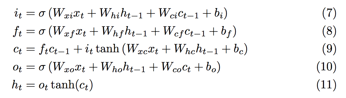
Here I will highlight some of my implementation. Please refer to the full script to see how data is loaded and training is done.
Creating a memory cell is substantially more involved than an RNN unit:
function addUnit(prev_h, prev_c, x, inputSize, hiddenSize)
  local ns = {}
  -- Input gate. Equation (7)
  ns.i_gate = nn.Sigmoid()(nn.CAddTable()({
    Linear(inputSize,hiddenSize)(x),
    Linear(hiddenSize,hiddenSize)(prev_h),
    Linear(hiddenSize,hiddenSize)(prev_c)
  }))
  -- Forget gate. Equation (8)
  ns.f_gate = nn.Sigmoid()(nn.CAddTable()({
    Linear(inputSize,hiddenSize)(x),
    Linear(hiddenSize,hiddenSize)(prev_h),
    Linear(hiddenSize,hiddenSize)(prev_c)
  }))
  -- New contribution to c. Right term in equation (9)
  ns.learning = nn.Tanh()(nn.CAddTable()({
    Linear(inputSize,hiddenSize)(x),
    Linear(hiddenSize,hiddenSize)(prev_h)
  }))
  -- Memory cell. Equation (9)
  ns.c = nn.CAddTable()({
    nn.CMulTable()({ns.f_gate, prev_c}),
    nn.CMulTable()({ns.i_gate, ns.learning})
  })
  -- Output gate. Equation (10)
  ns.o_gate = nn.Sigmoid()(nn.CAddTable()({
    Linear(inputSize,hiddenSize)(x),
    Linear(hiddenSize,hiddenSize)(prev_h),
    Linear(hiddenSize,hiddenSize)(ns.c)
  }))
  -- Updated hidden state. Equation (11)
  ns.h = nn.CMulTable()({ns.o_gate, nn.Tanh()(ns.c)})
  return ns
end
The crux of the code to string memory cells together is rather straightforward, it is parameterized by inputSize and hiddenSizes. This version handles creating an LSTM with one layer:
-- This will be the initial h (probably set to zeros)
ns.initial_h = nn.Identity()()
ns.initial_c = nn.Identity()()

-- The length indicators is a one-hot representation of where each sequence
-- ends. It is a BxL matrix with exactly one 1 in each row.
ns.lengthIndicators = nn.Identity()()

-- This will be expecting a matrix of size BxLxI where B is the batch size,
-- L is the sequence length, and I is the number of inputs.
ns.inputs = nn.Identity()()
ns.splitInputs = nn.SplitTable(2)(ns.inputs)

-- We Save all the hidden states in this table for use in prediction.
ns.hiddenStates = {}

-- Iterate over the anticipated sequence length, creating a unit for each
-- timestep.
local unit = {h=ns.initial_h, c=ns.initial_c}
for t=1,maxLength do
  local x = nn.SelectTable(t)(ns.splitInputs)
  unit = addUnit(unit.h, unit.c, x, inputSize, hiddenSize)
  -- We prepare it to get joined along the time steps as the middle dimension,
  -- by adding an middle dimension with size 1.
  print("timestep " .. t .. ", batchsize: " .. batchSize .. ", hiddenSize " .. hiddenSize)
  ns.hiddenStates[t] = nn.Reshape(batchSize, 1, hiddenSize)(unit.h)
end

-- INSERT CODE FRAGMENT X (above) HERE (omitted for brevity).

-- Combine into a single graph
local mod = nn.gModule({ns.initial_h, ns.initial_c, ns.inputs, ns.lengthIndicators},{ns.y})
And we’ll also need to share parameters among memory cells. You might have noticed I’ve been using a global function, Linear, but the name is not prefixed with nn, but it seems to work the same as nn.Linear. This is for the purpose of setting up parameter sharing. My function masquerading as nn.Linear keeps a table of all the linear modules while constructing the net, so that we have references to them later to set up parameter sharing:
LinearMaps = {}
Linear = function(a, b)
  local mod = nn.Linear(a,b)
  table.insert(LinearMaps, mod)
  return mod
end
We can then use this list to tie the 11 Linear maps of each Memory cell back to the first one:
-- Set up parameter sharing.
for t=2,numInput do
  for i=1,11 do
    local src = LinearMaps[i]
    local map = LinearMaps[(t-1)*11+i]
    local srcPar, srcGradPar = src:parameters()
    local mapPar, mapGradPar = map:parameters()
    mapPar[1]:set(srcPar[1])
    mapPar[2]:set(srcPar[2])
    mapGradPar[1]:set(srcGradPar[1])
    mapGradPar[2]:set(srcGradPar[2])
  end
end
Training and performance
LSTMs have many more parameters than our simple RNN, mainly do to all the additional parameter matrices involved in the input, forget, and output gates, and also because they have both a hidden state and a memory cell. So where our RNN with h=26 had 755 parameters, our LSTM with h=16 has 2049.
The performance looks very good.
This first plot is using the same fixed-width data set as our RNN example and using an LSTM implementation that doesn’t have the extra units to extract each batch member’s terminal hidden state, it can simply used the last hidden state for all batch members because they’re all the same length.

This LSTM converges nearly 2x as fast as the RNN despite all the additional parameters.
After adding our kludge for variable length sequences (in this script), we get similar results:
