Multi-layer perceptron
Introduction to neural nets with torch
Torch includes a very elegant collection of abstractions for building neural networks of various topologies (torch/nn). Because the components have a relatively uniform interface and fit together in standard ways, it straightforward to make all sorts of network topologies that Just Work™.
Each component compartmentalizes the details of how outputs are computed from inputs and how to back-propagate error signals. Thus when using pre-built components one merely needs to connect them together and all the details of forward and backward propagation are handled automatically and (usually) without error. In my experience I rarely have trouble with my gradients not being correct given the topology, my errors are usually in specifying the incorrect topology (or other issues like whether parameter sharing is set up properly, etc.).
The nn modules are more than neural net components, they are powerful, general purpose tools for computing with matrices and tables of matrices.
Here’s a sampling computations for which there are nn modules:
- linear transformation
- component-wise multiplication, or division
- addition of or multiplication a scalar
- propagate only a subset of columns or rows, reshape a tensor, or replicate inputs
- max, min, mean, sum, exp, abs, power, sqrt, square, normalize, etc.
- dropout
- join, split, subset or flatten tables
- mixture of experts
- dot product, cosine distance
- element-wise addition, subtraction, multiplication, division of tensors in a table
- convolution of all sorts
I will use the module for doing a linear map as an example. I will use a context (computer graphics) to illustrate that these modules can be used for general purpose computation, not just neural nets.
Here’s a matrix that represents clockwise rotation by 90° and a point at coordinates (2,0):
th> rotate = torch.Tensor{{0,1},{-1,0}}
 0  1
-1  0
[torch.DoubleTensor of size 2x2]
th> x = torch.Tensor{2,0}
 2
 0
[torch.DoubleTensor of size 2]
We can then declare a linear map nn module, copy in the parameters for our linear map (setting the bias to zero):
m = nn.Linear(2,2)
m:parameters()[1]:copy(rotate)
m:parameters()[2]:zero()
Now, when we do forward propagation, we simply performing matrix multiplication, in this case, causing our vector to rotate 90° clockwise:
th> m:forward(x)
 0
-2
[torch.DoubleTensor of size 2]
A classic feed-forward, MLP
Setting up a basic neural net is very simple:
num_inputs = 3
-- I pick this odd hidden layer size to result in the same number of parameters
-- as the two-layer example later.
h_size = 152
mlp = nn.Sequential()
mlp:add(nn.Linear(num_inputs, h_size))
mlp:add(nn.Sigmoid())
mlp:add(nn.Linear(h_size, 1))
The nn package contains a number of objective functions, including mean squared error and cross entropy. Since the target of our toy model is real-valued, we’ll use least-square loss:
criterion = nn.MSECriterion()Now we can set up a trainer to use stochastic gradient descent:
-- Set up a SGD trainer.
trainer = nn.StochasticGradient(mlp, criterion)
trainer.maxIteration = 50
We can then train the model, first setting initial parameters:
-- Get all the parameters packaged into a vector so we can reset them. It is important
-- to save a reference to this memory, because each call of getParameters() may
-- put the memory into new storage location.
mlp_params = mlp:getParameters()
mlp_params:uniform(-0.1, 0.1)
-- Train the model, after randomly initializing the parameters and clearing out
-- any existing gradient.
trainer:train(dataset)
The above model has 761 parameters. I run it with a batch size of 20, 70,000 training examples, a learn rate of 0.05, and 50 epoch (full code). Despite having lots of parameters and plenty of time to converge, it doesn’t do real well:
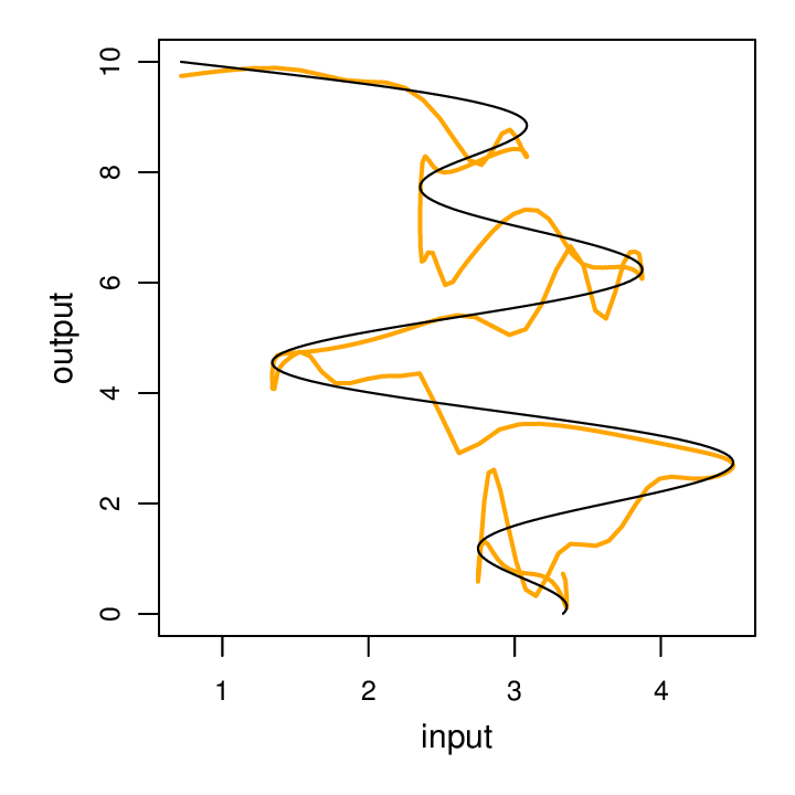
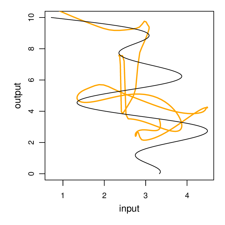
Yoshua Bengio suggests that we should pick the highest learn rate that doesn’t result in divergence, and that generally this is within a factor of two of the optimal learn rate. For the above, I selected a learn rate of 0.05. If we go just a little bit higher, to 0.06, all hell breaks lose:
It’s a very straightforward extension to add a second layer:
num_inputs = 3
h1_size = 30
h2_size = 20
mlp = nn.Sequential()
mlp:add(nn.Linear(num_inputs, h1_size))
mlp:add(nn.Sigmoid())
mlp:add(nn.Linear(params.h1, h2_size))
mlp:add(nn.Sigmoid())
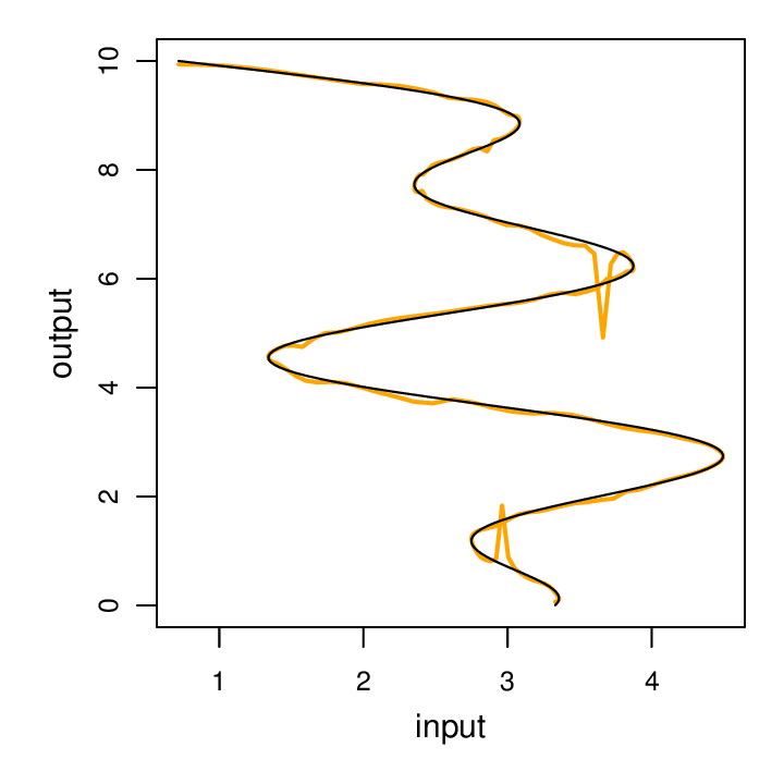
mlp:add(nn.Linear(h2_size, 1))This model also has 761 parameters. I train it with the same training data, batch size (20), learn rate (0.05) and number of epochs (50) as before. Interestingly, this performs much better, with just a few places where it gets confused:
While a classic feed-forward, multi-layer perceptron performs well on this toy problem, it’s not very flexible because it can’t handle varying-length sequences.