RNN

A major limitation of the feed-forward MLP architecture is that all examples must have the same width. This limitation can be overcome using various recurrent architectures.

In this example, we’ll build a single-layer recursive neural net. We’ll reuse the simulated toy data that we trained the MLP on, which happen to all have the same width, but generally recurrent neural nets will be used on sequences of varying lengths.

nngraph

We did reasonably well using the stock nn library to build a simple MLP. However, for more complicated architectures, the nngraph package offers an additional layer abstraction that proves quite useful. If you’re not familiar with nngraph you may want to see my brief introduction.

RNN implementation

Here’s what our toy RNN should look like unrolled:

The components that nn uses to build graphs are a bit more basic, and thus more flexible. The overall topology is the same, but there’s a few more pieces so that the tensors and tables are manipulated in the expected way. Here’s a visualization of the same RNN but using nn notation:

In practice, we want to abstract the length of the sequence to be any arbitrary length (up to a pre-defined maximum). So we’ll code building the RNN with a loop. Here we set len=3 so that the result matches the figure:

ni = 1; nh = 8; no = 1; len = 3
h0 = nn.Identity()()
x = nn.Identity()()
xs = nn.SplitTable(2)(x)
h = h0
for i=1,len do
  h = nn.Tanh()(nn.Linear(ni+nh,nh)(nn.JoinTable(1)({h,nn.SelectTable(i)(xs)})))
end
y = nn.Linear(nh,no)(h)
rnn = nn.gModule({h0,x},{y})

10 lines of code isn’t bad for an RNN, no? For our actual implementation, we’ll need to take care of a few more details. These include:

Setting up the network to work with mini-batches.
Sharing (tying) parameters among RNN units.
Getting our parameters all into one contiguous, linear vector for easy training updates.

Mini-batches

In some cases, nn.Modules work with mini-batches or single examples. This is sometimes possible by inspecting dimensions and lengths of tensors and assuming that if a tensor is one dimension short and too long, and would fit nicely by adding an extra dimension, it is assumed that this extra dimension iterates over the batches.

However in some cases additional explicit arguments are needed. For example, below we’ll pass an extra argument to JoinTable(2,2). This is all documented or readily apparent from the nn source.

All nn.Module instances can return a table of parameter tensors using mod:parameters(). nngraph nn.gModule instances also have a mod:parameter() function, but instead it returns a table of all parameter tensors for all modules in the graph.

When we inspect the parameters, we’ll see that the first two tensors look like the weight matrix and bias vector for the Linear(9,8) module. We have three such maps, explaining the first six. The final two are the weight matrix and bias vector for the Linear(8,1) mapping the terminal hidden state to the output variable, y.

th> p, gp = rnn:parameters()
th> p
{
  1 : DoubleTensor - size: 8x9
  2 : DoubleTensor - size: 8
  3 : DoubleTensor - size: 8x9
  4 : DoubleTensor - size: 8
  5 : DoubleTensor - size: 8x9
  6 : DoubleTensor - size: 8
  7 : DoubleTensor - size: 1x8
  8 : DoubleTensor - size: 1
}

Two values are returned from parameters(), the second is a table of all the gradient parameters. These also need to be shared so that as each unit accumulates the gradient during back-propagation, they’re all accumulating the gradient of one set of parameters.

We can tie the parameters together as follows:

  paramsTable, gradParamsTable = rnn:parameters()
  for t=2,length do
    -- Share weights matrix
    paramsTable[2*t-1]:set(paramsTable[1])
    -- Share bias vector
    paramsTable[2*t]:set(paramsTable[2])
    -- Share weights matrix gradient estimate
    gradParamsTable[2*t-1]:set(gradParamsTable[1])
    -- Share bias vector gradient estimate
    gradParamsTable[2*t]:set(gradParamsTable[2])
  end

Vectorizing parameters

In order to allow one training algorithm to work with pretty much any network architecture, we simply need to vectorize our parameters. Since all the parameters are unrolled into a single vector, we don’t need to know anything about the topology.

We can get parameters as follows:

  par, gradPar = rnn:getParameters()

We have one vector for the parameters and one vector for the gradient of the objective wrt the parameters. This function allocates a single contiguous chunk of memory for all the parameter tensors. Then the original parameter tensors are pointed back to this memory (which is just a matter of configuring the pointer and the stride). Because new memory is allocated, be sure not to run this function more than once, as any old references will no longer point to the actual tensors used.

Having vectorized parameters makes it easy to assign an initial guess:

  par:uniform(-0.1, 0.1)

And easy to perform an update:

  par:add(gradPar:mul(-learnRate))

Full implementation

Now with the above considerations in mind, here’s the crux of the RNN setup code, which is part of a larger script that handles data prep and draining.

function addUnit(prev_h, x, inputSize, hiddenSize)
  local ns = {}
  -- Concatenate x and prev_h into one input matrix. x is a Bx1 vector and
  -- prev_h is a BxH vector where B is batch size and H is hidden size.
  ns.phx = nn.JoinTable(2,2)({prev_h,x})
  -- Feed these through a combined linear map and squash it.
  ns.h = nn.Tanh()(nn.Linear(inputSize+hiddenSize, hiddenSize)({ns.phx}))
  return ns
end

-- Build the network
function buildNetwork(inputSize, hiddenSize, length)
  -- Keep a namespace.
  local ns = {inputSize=inputSize, hiddenSize=hiddenSize, length=length}

  -- This will be the initial h (probably set to zeros)
  ns.initial_h = nn.Identity()()

  -- This will be expecting a matrix of size BxLxI where B is the batch size,
  -- L is the sequence length, and I is the number of inputs.
  ns.inputs = nn.Identity()()
  ns.splitInputs = nn.SplitTable(2)(ns.inputs)

  -- Iterate over the anticipated sequence length, creating a unit for each
  -- timestep.
  local unit = {h=ns.initial_h}
  for i=1,length do
    local x = nn.Reshape(1)(nn.SelectTable(i)(ns.splitInputs))
    unit = addUnit(unit.h, x, inputSize, hiddenSize)
  end

  -- Output layer
  ns.y = nn.Linear(hiddenSize, 1)(unit.h)

  -- Combine into a single graph
  local mod = nn.gModule({ns.initial_h, ns.inputs},{ns.y})

  -- Set up parameter sharing. The parameter tables will each contain 2L+2
  -- tensors. Each of the first L pairs of tensors will be the linear map
  -- matrix and bias vector for the recurrent units. We'll link each of
  -- these back to the corresponding first one. 
  ns.paramsTable, ns.gradParamsTable = mod:parameters()
  for t=2,length do
    -- Share weights matrix
    ns.paramsTable[2*t-1]:set(ns.paramsTable[1])
    -- Share bias vector
    ns.paramsTable[2*t]:set(ns.paramsTable[2])
    -- Share weights matrix gradient estimate
    ns.gradParamsTable[2*t-1]:set(ns.gradParamsTable[1])
    -- Share bias vector gradient estimate
    ns.gradParamsTable[2*t]:set(ns.gradParamsTable[2])
  end

  -- These vectors will be the flattened vectors.
  ns.par, ns.gradPar = mod:getParameters()
  mod.ns = ns
  return mod
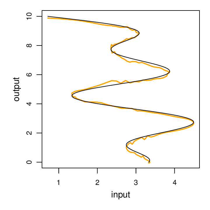
end

How does it fare? Well, when we train it as follows:

th model-1_layer.lua -hidden 26 -batch 20 -rate 0.02 -iter 30

We can see it does quite well. The model has 755 parameters, which is comparable to our MLP implementations.

Now that we have a simple RNN under our belt, lets enhance it a bit by turning it into an LSTM.

up next: LSTM

nngraph

RNN implementation

Mini-batches

Parameter sharing

Vectorizing parameters

Full implementation