Toy problem

When I first started learning about neural nets, I found the 1 dimensional example of a neural net learning an arbitrary function not only good for building intuition, but helpful for testing initial implementations I coded up to learn.

Here I take a similar approach, but since we want to understand LSTMs, which are used for modeling sequential data, we would like to create a toy problem for which sequential information is important to successfully modeling it.

Here I use a weighted average of four arbitrary functions sine waves to come up with a mapping:

f = function(x) return (
  torch.sin(x/2 - 1):mul(0.5) +
  torch.sin(x) +
  torch.sin(x*2 + 2) +
  torch.sin(x/4 + 1) + 2)
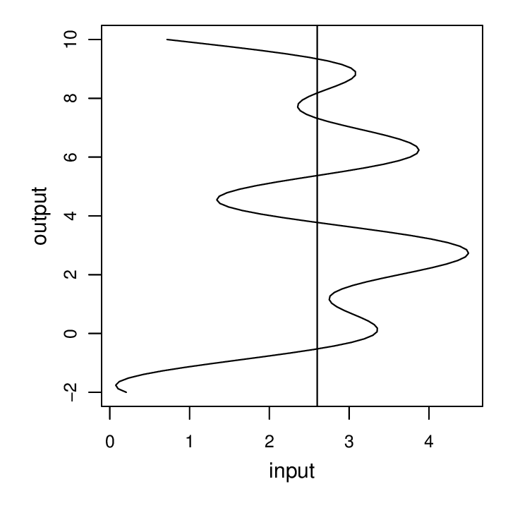
end

This will result in a somewhat wavy function, and by considering the inverse mapping, we get a modeling problem whereby a single input (horizontal axis) doesn’t uniquely define the output (vertical axis), as illustrated by the vertical line which crosses the curve in six places:

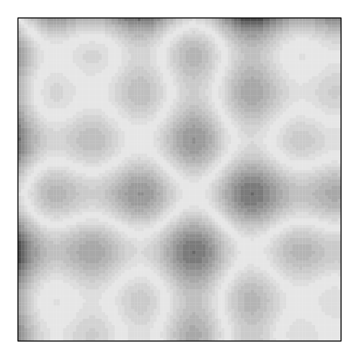
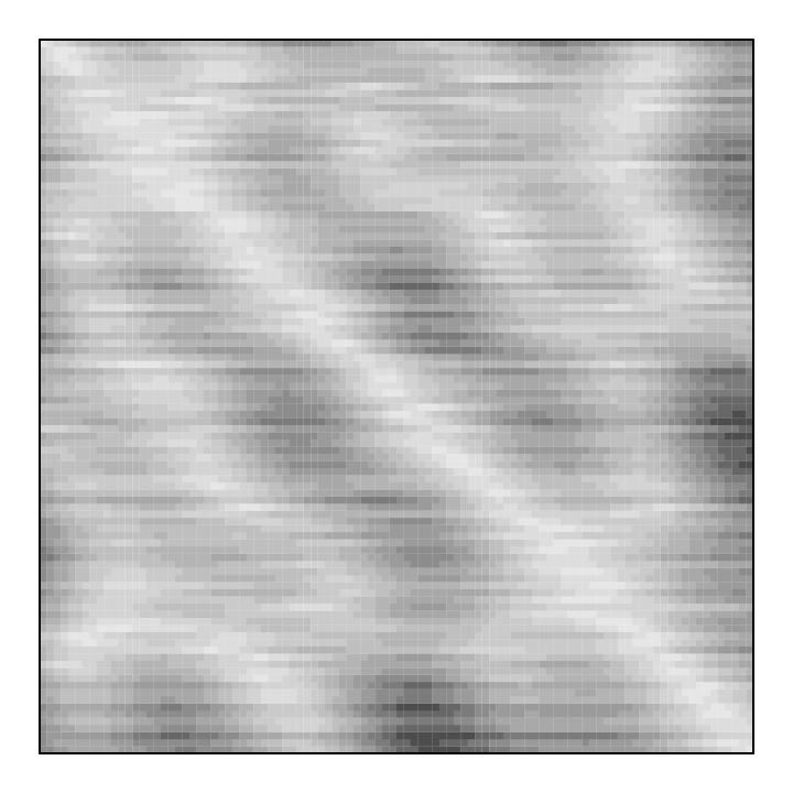
Another way to visualize this being not uniquely determined is to consider how similar inputs are to each other even when they correspond to outputs that are far apart. The following figure shows how similar each input is to each other input. The grayscale intensity is |f(z)-f(z’)| and the axes are z and z’. The point is to illustrate why learning a mapping that is not one-to-one is challenging and would benefit from sequential information. Consider a point on the horizontal axis, z. There are several values of z’ on the vertical axis that produce f(z) - f(z’) near zero (white). Thus, if you have a value, a = f(z), and you want to feed this to your neural net to get back z, it’s non-identifiable. As expected, the diagonal is perfectly similar to itself (white), but there are plenty of off-diagonal similar cells to make the mapping confusing:

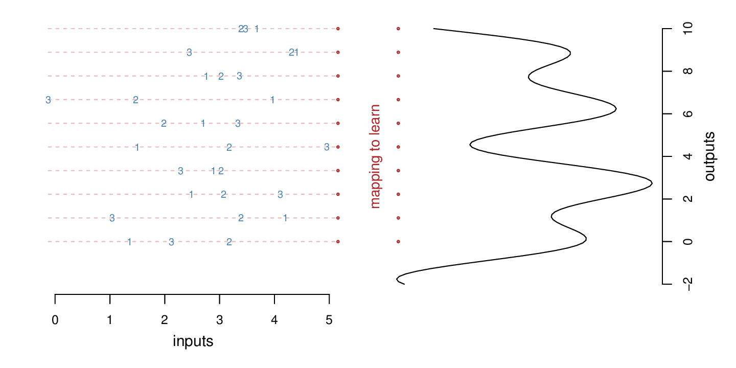
In order to make the problem more solvable and relevant to RNN and LSTM neural nets, we add a sequential aspect to this modeling problem, considering three inputs instead of one. One (arbitrary) way to do this is to consider three evenly spaced points in the original mapping: z, z-1, z-2 (z is the vertical position marked with a dotted line in the next figure). Each of these can be transformed by our function with some noise added: (f(z)+e f(z-1)+e, f(z-2)+2) where e ~ N(0, 0.16). We then can consider these three values as the inputs, and our goal is to predict what is the original z:

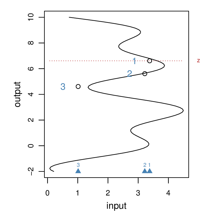
In the above plot, the inputs are marked by the three blue triangles at the bottom. The output we’re trying to predict is the red dotted line at z. The inputs are derived by adding two points evenly spaced below z, computing their corresponding f(z) values and adding some noise.

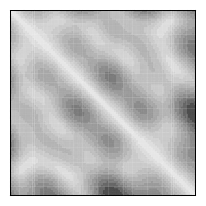
Instead of having just one point a = f(z), we have a vector values, (a, b, c), where we know that these must have been produced by some f(z), f(z-1), f(z-2). This problem is much easier. We can illustrate using a similar figure to one above. In this next figure, the grayscale intensity is the Euclidean distance between (f(z), f(z-1), f(z-2)) and (f(z’), f(z’-1), f(z’-2)). Now the diagonal is much more prominent and the sequential information is clearly helping.

By having access to a sequence of three inputs we now can get a better idea of what part of the curve these must have been derived from. In this way, the sequential information provides context and should enable us to solve the inverse mapping problem. With a single input, we would only know the location of the gray line, which crosses the curve at six places. But with the three ordered triangles, there is much less ambiguity that these points must have been derived from z (red dotted line), even despite the additional noise.

It’s worth noting that the above figure is without any noise. If we add some noise to the inputs, the problem gets a bit harder. The diagonal is still apparent, but much less clear:

In the next figure, we see 10 examples that may give us a better idea of the prediction problem with which we’ll be faced. On the left, I have permuted the rows so that we can’t immediately see the corresponds between the left and the curve on the right. Our goal is to learn the mapping connecting the red dots on the left with the red dots on the right.

Try for a moment to do the mapping in your head by visual inspection.

While not terribly difficult, it takes some thinking and a few tries.

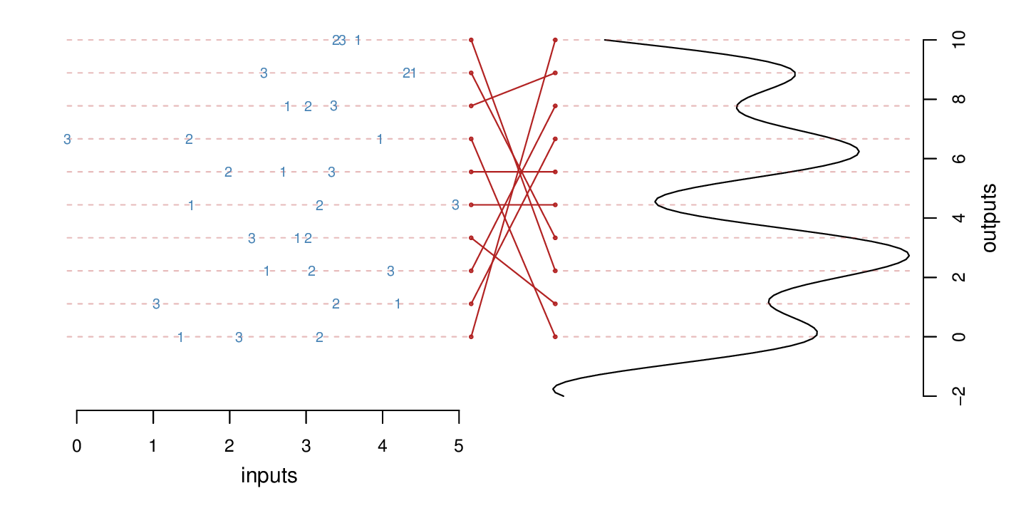
In this next figure, I fill in the mapping. Now the red dots on the left are connected to the z locations along the curve from which the “1” points are derived. The “2” and “3” points then correspond to the locations on the curve at offset distances of 1 and 2 below the focal point.

We will use this toy problem, and slight variations to explore classic feed-forward neural nets (multi-layer perceptrons / MLP), recursive neural nets (RNN), and long-term short-term memory neural nets (LSTM).